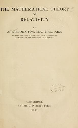
The Mathematical Theory of RelativityEddington, Arthur Stanley, Sir
Science
The Mathematical Theory of Relativity
Eddington, Arthur Stanley, Sir
Relativity (Physics)
Take a point on the surface as origin. Let $(x_{1}, x_{2}, x_{3}, x_{4})$ be rectangular
coordinates in the tangent plane (four-dimensional) at the origin; and let the
fifth rectangular axis along the normal be~$z$. Then by Euclidean geometry
\[
-ds^{2} = dx_{1}^{2} + dx_{2}^{2} + dx_{3}^{2} + dx_{4}^{2} + dz^{2},
\Tag{(65.1)}
\]
imaginary values of~$ds$ corresponding as usual to real distances in space. The
four-dimensional surface will be specified by a single equation between the
five coordinates, which we may take to be
\[
z = f(x_{1}, x_{2}, x_{3}, x_{4}).
\]
If the origin is a regular point this can be expanded in powers of the~$x$'s. The
deviation from the tangent plane is of the second order compared with distances
parallel to the plane; consequently $z$~does not contain linear terms in
the~$x$'s. The expansion accordingly starts with a homogeneous quadratic
function, and the equation is of the form
\[
2z = a_{\mu\nu} x_{\mu} x_{\nu},
\Tag{(65.2)}
\]
correct to the second order. For a fixed value of~$z$ the quadric~\Eq{(65.2)} is called
the \emph{indicatrix}.
\index{Indicatrix}%
The radius of curvature of any normal section of the surface is found by
the well-known method. If $t$~is the radius of the indicatrix in the direction of
the section (direction cosines $l_{1}$, $l_{2}$, $l_{3}$, $l_{4}$), the radius of curvature is
\[
\rho = \frac{t^{2}}{2z} = \frac{1}{a_{\mu\nu} l_{\mu} l_{\nu}}.
\]
In particular, if the axes are rotated so as to coincide with the principal axes
of the indicatrix, \Eq{(65.2)}~becomes
\[
2z = k_{1}\, dx_{1}^{2} + k_{2}\, dx_{2}^{2} + k_{3}\, dx_{3}^{2} + k_{4}\, dx_{4}^{2},
\Tag{(65.3)}
\]
and the principal radii of curvature of the surface are the reciprocals of
$k_{1}$, $k_{2}$, $k_{3}$,~$k_{4}$.
Differentiating~\Eq{(65.2)}
\[
dz = a_{\mu\nu} x_{\mu}\, dx_{\nu},\quad
dz^{2} = a_{\mu\nu} x_{\mu}\, dx_{\nu} · a_{\sigma\tau} x_{\sigma}\, dx_{\tau}.
\]
Hence, substituting in~\Eq{(65.1)}
\[
-ds^{2} = dx_{1}^{2} + dx_{2}^{2} + dx_{3}^{2} + dx_{4}^{2}
+ (a_{\mu\nu} a_{\sigma\tau} x_{\mu} x_{\sigma})\, dx_{\nu}\, dx_{\tau}
\]
for points in the four-dimensional continuum. Accordingly
\[
-g_{\nu\tau} = g_{\nu}^{\tau} + a_{\mu\nu} a_{\sigma\tau} x_{\mu} x_{\sigma}.
\Tag{(65.4)}
\]
Hence at the origin the~$g_{\mu\nu}$ are Euclidean; their first derivatives vanish;
and their second derivatives are given by
\[
\frac{\dd^{2} g_{\nu\tau}}{\dd x_{\mu}\, \dd x_{\sigma}}
= -(a_{\mu\nu} a_{\sigma\tau} + a_{\sigma\nu} a_{\mu\tau}),
\]
by~\Eq{(35.5)}.
Public-domain text, read in full here on John Shaqi.
Reviews
Reviews
No reviews yet
Be the first to share your thoughts on this work.
Elsewhere in the archive
Join the Discussion
Join the discussion
Sign in to leave a comment or review.
Sign InorCreate an account